Introduction

Time series analysis is a powerful tool used in various fields including finance, economics, engineering, and environmental science. It helps in understanding past patterns to forecast future trends, making it invaluable for decision-making. In this guide, we will explore the components of time series, moving averages, autocorrelation, and practical applications of these techniques.

Understanding Time Series

A time series is a sequence of data points collected at successive equally spaced time intervals. It is used to understand the past behavior of a phenomenon or to predict future behavior based on its historical data.

Characteristics and properties of time series data:

• Temporal Dependence: Data points are not independent; each value is dependent on previous values.
• Seasonality: Regular patterns that repeat at known intervals.
• Trend: Long-term movement indicating overall direction.
• Cyclicality: Fluctuations occurring at intervals not fixed or seasonal.

Examples of time series data:

• Stock Prices: Daily closing prices of stocks over time.
• Temperature: Daily temperature readings over a year.
• Sales: Monthly sales data of a product.

1. Time Series Components (Trend, Seasonality, Cyclicality)

Understanding the components of a time series is crucial for accurate analysis and forecasting. Let's delve into the key components: trend, seasonality, and cyclicality.

1.1 Trend

The trend component represents the long-term movement of a time series, indicating whether it is increasing, decreasing, or stable over time. Trends can be:

• Upward Trend: Values increase over time.
• Downward Trend: Values decrease over time.
• Stable Trend: Values remain relatively constant over time.

1.2 Examples:

• A company's stock price increasing steadily over the years.
• Population growth in a city over decades.

Trend analysis helps in understanding the underlying growth or decline of a phenomenon, which is essential for long-term planning and decision-making.

1.3 Seasonality

Seasonality refers to patterns that repeat at known regular intervals within the data. These patterns could be daily, weekly, monthly, or yearly. Seasonal patterns are influenced by factors such as weather, holidays, and cultural events.

1.4 Examples:

• Sales of winter clothing increasing during the colder months.
• Increase in retail sales during the holiday season.

Identifying seasonality helps in predicting short-term fluctuations and adjusting strategies accordingly. Seasonal adjustments are often used to remove these patterns to reveal underlying trends.

1.5 Cyclicality

Cyclicality involves fluctuations in the data that occur at intervals longer than those of seasonality. Unlike seasonal patterns, cyclic patterns are not fixed and can vary in duration and intensity.

1.6 Examples:

• Business cycles with periods of expansion and contraction.
• Economic cycles affecting employment rates and inflation.

Understanding cyclicality helps in predicting medium-term fluctuations in the data and is crucial for adjusting economic policies and business strategies.

1.7 Importance in Time Series Analysis

Accurately identifying and separating these components is essential for developing robust forecasting models. Techniques such as decomposing time series into trend, seasonality, and residual components help in understanding the data's structure and making reliable predictions.

2. Moving Averages in Time Series Analysis

Moving averages are fundamental tools in time series analysis used to smooth out short-term fluctuations and highlight longer-term trends. Let's explore the concept of moving averages and their applications.

2.1 What is a Moving Average?

A moving average (MA) calculates the average of a series of data points over a specified period. It moves or "slides" across the data to create a series of averages. Moving averages are useful because they help to reduce the noise in the data and make it easier to spot trends over time.

2.2 Types of Moving Averages

There are several types of moving averages commonly used:

1. Simple Moving Average (SMA): The SMA calculates the average of a set number of periods equally.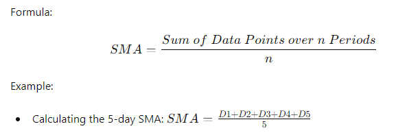

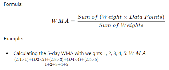
      2.    Weighted Moving Average (WMA): The WMA assigns weights to each data point based on its position in the series.

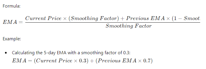
  3.    Exponential Moving Average (EMA): The EMA gives more weight to recent data points and is more responsive to recent price           changes.

2.3 Applications of Moving Averages

1. Trend Identification: Moving averages help in identifying trends by smoothing out short-term fluctuations.

2. Support and Resistance Levels: Moving averages can act as dynamic support and resistance levels.

3. Crossover Signals: Crossovers between different moving averages (e.g., SMA and EMA) can signal potential buy or sell opportunities.

4. Forecasting: Moving averages are used in time series forecasting models to predict future trends.

2.4 Choosing the Right Moving Average

The choice of moving average depends on the specific application and the characteristics of the data. Shorter-term moving averages are more sensitive to price changes, while longer-term moving averages are smoother and less responsive to price fluctuations.

2.5 Example Application

Let's consider an example of using a moving average to analyze stock prices:

• Objective: Analyze the trend in the stock price of Company X over the past 50 days.
• Method: Calculate the 50-day SMA and plot it against the daily closing prices.

By applying a 50-day SMA, we can smooth out the daily fluctuations and identify the overall trend in the stock price.

3. Autocorrelation in Time Series Analysis

Autocorrelation is a crucial concept in time series analysis that measures the degree of similarity between a time series and a lagged version of itself over successive time intervals. Let's delve into what autocorrelation is, how it is calculated, and its significance in analyzing time series data.

3.1 What is Autocorrelation?

Autocorrelation measures how a time series is correlated with a lagged version of itself. In simpler terms, it checks if the values of the time series data points are related to previous data points.

3.2 Types of Autocorrelation

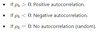
1. Positive Autocorrelation: This occurs when a time series data point is positively correlated with a previous data point.

2. Negative Autocorrelation: This occurs when a time series data point is negatively correlated with a previous data point.

3. Zero Autocorrelation: This occurs when there is no correlation between a time series data point and a previous data point.

3.3 How is Autocorrelation Calculated?

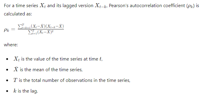
Autocorrelation is calculated using a mathematical formula. The most commonly used method to measure autocorrelation is Pearson's correlation coefficient.

3.4 Significance of Autocorrelation

Autocorrelation is significant for several reasons in time series analysis:

1. Identifying Patterns: It helps to identify patterns and trends in the time series data.

2. Modeling: Autocorrelation is used in modeling time series data for forecasting future values.

3. Stationarity: Autocorrelation can indicate if a time series is stationary or non-stationary.

4. Diagnostics: It is used as a diagnostic tool for checking assumptions in time series models.

3.5 Interpretation of Autocorrelation

3.5`Example Application

Let's consider an example to illustrate autocorrelation in stock prices:

• Objective: Analyze the autocorrelation of the daily closing prices of Company Y over a lag of 10 days.
• Method: Calculate the autocorrelation coefficient (p10) and interpret the results.

By applying autocorrelation analysis, we can understand how closely today's stock prices are related to the prices of the previous 10 days.

Conclusion

In conclusion, this comprehensive guide has explored various essential aspects of time series analysis, focusing on key components such as trend, seasonality, moving averages, and autocorrelation. We've covered how each of these components contributes to understanding and forecasting time-dependent data.

Time Series Analysis and StocksPhi

Throughout this article, we've seen how crucial time series analysis is for traders, investors, learners, technologists, and professionals in making informed decisions. StocksPhi provides advanced tools and expertise in time series analysis, helping traders and investors navigate the complexities of financial markets.

From identifying trends and seasonality to using moving averages and understanding autocorrelation, StocksPhi offers sophisticated solutions that empower users to analyze data effectively. By leveraging StocksPhi's services, traders can gain deeper insights into market patterns and optimize their trading strategies.

Key Takeaways

1. Trend: Identifying the long-term direction of a time series.
2. Seasonality: Understanding periodic fluctuations in time series data.
3. Moving Averages: Smoothing out short-term fluctuations to identify trends.
4. Autocorrelation: Measuring the similarity between a time series and a lagged version of itself.

Why Time Series Analysis Matters

• Forecasting: Predicting future values based on historical data.
• Decision-Making: Supporting informed decisions in trading and investment.
• Pattern Recognition: Identifying repeating patterns and anomalies.