Introduction 

Probability distributions form the backbone of quantitative analysis. They offer a mathematical framework to quantify the likelihood of various outcomes across different scenarios. Mastering these distributions is vital for making informed decisions in fields such as finance, engineering, healthcare, and social sciences. This guide delves into four crucial probability distributions: Normal, Binomial, Poisson, and Exponential, and highlights their applications in quantitative analysis.

Understanding Probability Distributions

Probability distributions are mathematical functions that describe the probabilities of various outcomes for a random variable. These distributions provide valuable insights into data spread and shape, helping analysts and researchers navigate uncertainty and variability in datasets. Each distribution has unique parameters and characteristics that define its behavior.

Normal Distribution

Grasping the Normal Distribution

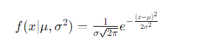
The Normal distribution, also known as the Gaussian distribution, is the most widely recognized distribution in statistics. It is depicted by a symmetric bell-shaped curve centered around its mean.

The formula for the probability density function (PDF) of the Normal distribution is:

• Mean (μ): Determines the center of the distribution.

• Standard Deviation (σ): Measures the spread of the distribution.

The Empirical Rule (68-95-99.7 Rule):

• About 68% of data falls within one standard deviation of the mean.
• About 95% falls within two standard deviations.
• About 99.7% falls within three standard deviations.

Calculating Probabilities with the Normal Distribution

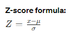
To calculate probabilities, we use the Z-score, which indicates how many standard deviations an element is from the mean.

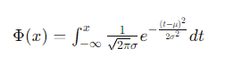
Cumulative Distribution Function (CDF):

The CDF provides the probability that a random variable 𝑋   will take a value less than or equal to 𝑥 .

Examples and Applications

• Example: Heights of individuals in a population with a mean height of 170 cm and a standard deviation of 10 cm. Calculate the probability of finding someone with a height between 160 cm and 180 cm.
• Real-world applications:
  • Finance: Modeling stock market returns.
  • Quality Control: Analyzing production processes.

Binomial Distribution

Understanding the Binomial Distribution

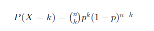
The Binomial distribution models the number of successes in a fixed number of independent Bernoulli trials, each with the same probability of success.

The probability mass function (PMF) of the Binomial distribution is:

• n: Number of trials.
• k: Number of successes.
• p: Probability of success in each trial.

Characteristics and Parameters

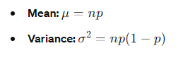
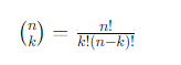
Calculating Binomial Probabilities

Binomial coefficient:

Cumulative Distribution Function (CDF):

𝐹(𝑘;𝑛,𝑝)=∑𝑖=0𝑘(𝑛𝑖)𝑝𝑖(1−𝑝)𝑛−𝑖

Examples and Applications

• Example: Flipping a coin 10 times, where success is getting heads. Calculate the probability of getting exactly 5 heads.
• Real-world applications:
  • Quality Control: Assessing defective products in a batch.
  • Marketing: Measuring response rates to a campaign.

Poisson Distribution

Grasping the Poisson Distribution

The Poisson distribution expresses the probability of a given number of events occurring within a fixed interval of time or space.

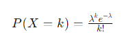
The probability mass function (PMF) of the Poisson distribution is:

𝑃(𝑋=𝑘)=𝜆𝑘𝑒−𝜆𝑘!

• λ: Average rate of occurrences.
• k: Number of occurrences.

Characteristics and Parameters

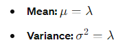
Calculating Poisson Probabilities

Cumulative Distribution Function (CDF):

 Examples and Applications

• Example: Number of emails received per hour, with 𝜆=5 λ = 5 . Calculate the probability of receiving exactly 3 emails in an hour.
• Real-world applications:
  • Traffic Flow: Counting cars passing through a toll booth per hour.
  • Biology: Tracking mutations on a DNA strand.

Exponential Distribution

Understanding the Exponential Distribution

The Exponential distribution describes the time between events in a Poisson process, where events occur continuously and independently at a constant average rate.

Characteristics and Parameters

​

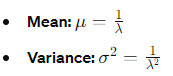
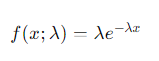
Probability Density Function (PDF):

𝑓(𝑥;𝜆)=𝜆𝑒−𝜆𝑥

• λ: Rate parameter.
• x: Time between events.

Calculating Exponential Probabilities

Cumulative Distribution Function (CDF):

𝐹(𝑥;𝜆)=1−𝑒−𝜆𝑥

Examples and Applications

• Example: Time until the next radioactive decay event, with 𝜆=0.1 λ = 0.1 decays per minute. Calculate the probability that the next decay occurs within the next 5 minutes.
• Real-world applications:
  • Queueing Theory: Modeling waiting times.
  • Reliability Engineering: Estimating the lifetime of electronic components.

Conclusion

Grasping the concepts of probability distributions—specifically the Normal, Binomial, Poisson, and Exponential distributions—is essential for anyone involved in quantitative analysis and statistical methods. Each distribution serves unique purposes and finds applications across various fields, making them indispensable tools in statistical analysis.